Building a Predictive Maintenance Logger for My Haltech Rebel LS

Why I built this

My Haltech Rebel LS is a fully programmable ECU on a supercharged LS V8. It monitors everything — injector current per cylinder, ignition coil voltage, knock sensors, lambda, fuel pressure, coolant temp, manifold pressure, RPM — and it has a built-in Wi-Fi access point that broadcasts this data over UDP.

The obvious thing: log it all and watch for trouble. The problem is volume: at ~10 Hz across 1,000 channels, a 20-minute track session generates 35–60 MB of raw data. Tens of millions of data points per session. How do you find the signal in that noise?

There’s also a hard constraint I didn’t fully appreciate at first. The published research on injector diagnostics describes fault signatures that need 100 kS/s (10 µs resolution) — needle displacement reducing peak current by 35%, coil charging delay increasing by 0.2 ms. We poll at ~10 Hz. That means we cannot reconstruct injector current waveforms, misfire profiles from crank acceleration, or any per-combustion-event signal.

But the ECU already does that internally and exposes the results as derived scalars: Injector N Current, Injection Stage 1 Dead Time, Flow Rate, misfire counters, knock levels. Our strategy is to log the ECU’s conclusions rather than try to reproduce its measurements. The achieved sample rate is recorded in every session’s metadata, and no detector runs if the rate cannot support it.

This is the story of how I reverse-engineered the protocol, built an Android app to pull it all down, and wrote a Python analysis pipeline that looks for two different kinds of failures — without drowning in data.

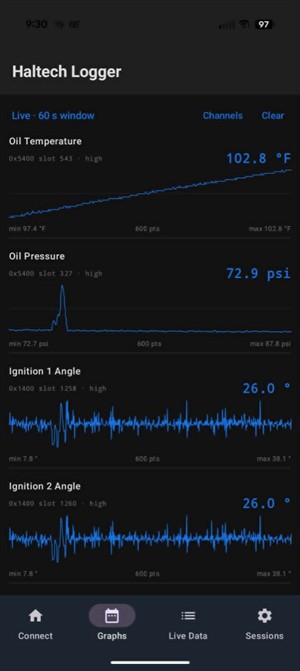Live Graphs screen. Named channels in engineering units (°F, psi, degrees), each with a rolling 60-second strip chart, min/max, and the ECU window/slot identity underneath.

Two kinds of failures

I realized early on that engine failures show up in two completely different ways, and they need different tools:

Failure mode	Timescale	Example	What it looks like
Sudden	Seconds to minutes within one session	An injector starts clogging mid-session, a coil breaks down	One cylinder’s injector current drops 8% below the other seven
Slow drift	Weeks to months across many sessions	Rod bearing clearance grows, fuel pump wears	Oil pressure at 4,000 RPM is 5% lower than it was 10 sessions ago

One detector cannot cover both. So the system has two separate analysis paths — and completely different storage strategies to support them.

How it works

The whole pipeline is just four layers:

Phone → Binary files → Python analysis → One-page summary

The app

The phone joins the ECU’s Wi-Fi (it broadcasts its own access point), polls it over a reverse-engineered UDP telemetry protocol, and writes every sample to a custom binary format (.hrlg). The format is self-describing — it carries the channel map inside it, so a session recorded today will still be readable years from now regardless of what app version wrote it.

What the app does today, on the car:

• Dual-window poll at ~10 Hz for the electrical / spark / knock window and ~5 Hz (held between refreshes) for the sensor / fuel / oil window — neither window is a superset of the other.
• Graphs in engineering units (°F, psi, λ, %). Manifold pressure is shown as gauge pressure (baro-corrected) so idle vacuum reads negative instead of looking like several psi of boost on a naturally aspirated engine.
• Session recording with on-device summarization, Room history, zip export, and playback of any saved session through the same graph UI (play/pause, scrub, 0.5–4×).
• DTC freeze-frame capture when a trouble code sets, with a timestamp.

The format makes three deliberate design decisions:

• Append-only: Frames are written as they arrive. A crash or dead battery loses only the tail, not the whole file.
• Channel identity, not slot index: Each entry stores the stable channel ID from the Haltech channel CSV, never the slot number. The slot layout can shift with ECU firmware or configuration changes — the channel ID cannot.
• Mapped channels only in frames: .hrlg v2 stores the mapped slot set (~410 channels), not every raw ECU word — roughly 1.6 KB/frame, ~12 MB for a 25-minute session at 10 Hz.

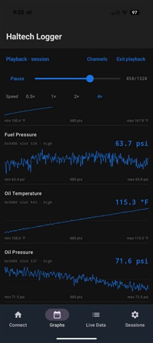Playback of a recorded session. Same strip charts as live; scrub the timeline and the trailing 60-second window rebuilds around that point.

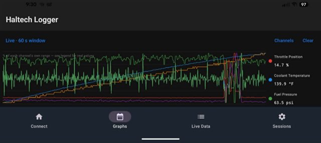Landscape mode overlays every selected channel on one chart. Units can’t share a single axis (RPM vs psi vs %), so each series is normalized to its own min/max for the plot; the legend carries the real values.

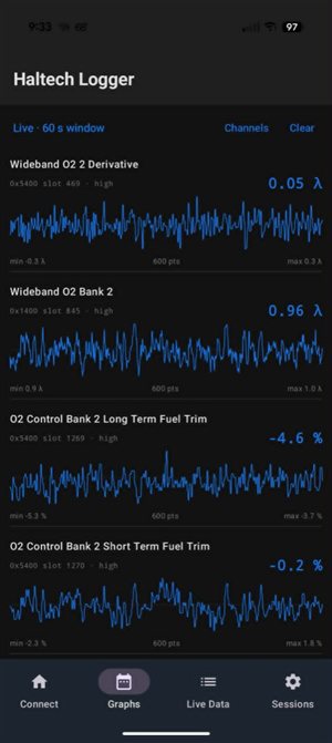Bank 2 wideband and fuel trims during a live poll — the same lanes the sudden-failure detectors will read from session exports.

At the end of a session, the app computes per-channel statistics: min, max, mean, p05, p50, p95, standard deviation, and sample count. That’s ~300 channels × 12 numbers = a few kilobytes per session. This is the only data that ever gets queried across sessions. The raw session file stays on-device (and can be exported as a zip).

Sudden-failure detection

The core technique is beautifully simple: compare each cylinder against the other seven.

If cylinder 3’s injector current is 8% below the average of cylinders 1, 2, 4, 5, 6, 7, and 8, that’s a signal — regardless of how hard you’re driving or what the fuel temperature is. No history needed, no calibration, no absolute thresholds.

This is the same principle as bilateral asymmetry monitoring used in aero-engine diagnostics — comparing symmetric halves of a jet engine to each other — applied at the cylinder level.

The math uses a MAD z-score (median absolute deviation), which is deliberately chosen over the standard z-score (mean and standard deviation). The reason: one failing injector pulls the mean toward it, hiding the failure. The median and MAD are resistant to a single outlier skewing the reference. A cylinder is only flagged if it stays anomalous for several consecutive samples — not just a single noise spike.

Dual-element sensors (throttle pedal A/B, throttle position A/B) get their own cross-check: the two channels should track each other linearly. A drop in correlation means the sensor is failing right now, before any DTC sets.

The system also monitors at the bank level: if the two wideband O2 sensor readings diverge but the fuel trims do not follow, the sensor is suspect — not the mixture. This is a cross-check no single channel can provide.

Slow-drift detection

Raw session averages are a trap. A session with more idling reads lower oil pressure; a session with more high-RPM pulls reads higher. Comparing averages across sessions measures driving style, not wear.

The fix is operating-point binning: every sample gets classified into a cell by (RPM range × engine load × temperature), and statistics are computed within each cell. Then the same cell is compared across sessions:

“Oil pressure p50 in the cell 4,000-4,500 RPM × 70-80% load was 52 psi for sessions 1-8, 50 psi for sessions 9-14, and 47 psi for sessions 15-20.”

That series is comparable. A raw session-mean would hide it entirely.

Data quality first. Before computing bin statistics, each bin’s samples are filtered for plausibility. A single torn read can poison a bin’s mean. The filter uses IQR (interquartile range) trimming: values outside Q1 - 1.5×IQR or Q3 + 1.5×IQR are excluded. Heavy trimming in a bin is itself a signal worth surfacing — it tells you the sensor is noisy.

Trend fitting. For each (channel × operating-point cell) with data across multiple sessions, a linear trend is fitted. A slope is flagged when two conditions hold: the fitted drift over the observed span exceeds the channel’s own natural variance, and the projection crosses a defined limit within a foreseeable number of sessions. Output is phrased as a finding with confidence bounds:

“Oil pressure p50 in the 4,000 RPM / 75% load cell declined 6% over 11 sessions; at this rate, it crosses the 40 psi advisory limit at session 24.”

Alongside the linear trend, a change-point detector looks for the session at which behavior began to shift. “The pump started degrading around session 14” is more useful than “there is a downward slope across all 20 sessions,” and is the established approach for remaining-useful-life estimation under variable operating conditions.

There’s also a hot-idle fingerprint: at the end of every session (fully warm, stable idle), I record oil pressure, manifold vacuum, fuel trims, and knock background level. One small, deliberately-revisited operating point is worth more for month-over-month comparison than the entire rest of the session. Rod bearing clearance growth shows up at hot idle first.

The maintenance log. A trend across a window that contains an unrecorded injector swap is not a trend. Every session record carries metadata for oil grade, parts replaced, compression test results, and oil analysis references. This is the cheapest thing to get right and the most expensive to reconstruct later.

The LLM summary

The LLM never sees raw data. Feeding raw numeric series to an LLM as text is counterproductive — the tokenizer splits 1024 into either 10 + 24 or 102 + 4 depending on training data, numeric precision suffers, and large contexts degrade model performance. This is a well-documented pattern in the literature (IJCAI 2024 survey on LLMs for time series).

Deterministic Python does all the arithmetic — extraction, z-score computation, binning, regression, event detection. The LLM sees only a compact, unit-labeled report. The model’s job is to correlate across subsystems — “cylinder 3 injector current is low and bank 1 fuel trim is positive and knock trim is retarding cylinder 3” — and produce a ranked list of what to inspect.

Every number carries units and a sample count: “Injector 3 current p50 = 0.71 A (n=3100)” — never a bare number. Findings are ranked, cite their source sessions and channels, and the output is always a “what to check” list, not a verdict. The human makes the final call.

The hardest part: the channel map

The ECU broadcasts data in a fixed set of memory-mapped slots. Only a subset are actually mapped to ECU channels, and the slot a channel lives in can shift between firmware versions. The mapping from slot to channel identity was worked out by correlating raw bytes against Haltech’s own PC software (NSP) CSV exports during known state changes — including an engine-running capture so RPM, MAP, oil, fuel pressure, and knock weren’t just coincidences from an engine-off session.

Every mapping carries a confidence level:

Confidence	What it means	What we do with it
CONFIRMED / high	Verified against NSP CSV or known state change	Include in detectors
TENTATIVE / medium	Plausible but not yet verified	Include but flag it
PENDING / not identified	In the CSV but not yet located in the window	Exclude entirely — never guess
COLLISION	Two channels map to the same slot	Exclude — ambiguous

We never act on a channel we’re not sure about. About 306 channels are confirmed across the two live windows the app polls. The Graphs picker only offers slots that actually exist in those windows — and anything still unidentified stays labelled that way rather than plotted as a misleading flat line.

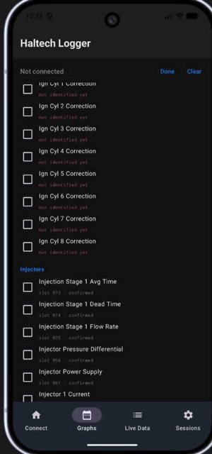Channel picker. Confirmed injector channels carry a slot; ignition corrections that aren’t mapped yet stay labelled “not identified yet” and never get treated as real data.

What I’d do differently

Verify bytes off the wire, not in a simulation. I spent a week debugging a protocol issue that didn’t exist in my Python model. The actual app was sending a wrong-sized request while my “proven” reference was actually a different size. The fix: capture the phone’s actual UDP traffic with tshark and compare against that — never against a filtered CSV extract. A later multi-second drop that looked like SoftAP corruption turned out to be a one-byte framing bug that only fired after a fixed number of transactions — same lesson, different week.

Never invent engineering-unit mappings from one capture. The first time I “confirmed” RPM, MAP, and TPS from a single engine-off session, all three were wrong — they were raw analogue input millivolts. Correlation against an NSP CSV with the engine running is the only source of truth.

Never compare session averages. Operating-point binning is the only way to get comparable numbers across sessions.

LLMs are synthesis tools, not data analysts. They’re terrible at reading raw numbers. Give them features, not samples.

Tune thresholds against real failures. All detection thresholds are currently provisional, calibrated against synthetic test data. The conscious decision is to run with deliberately conservative thresholds and tune them against real flagged events as they occur. There is no substitute for real failure data.

How to try the Android logger

I’m distributing time-limited loaner builds through Firebase App Distribution — R8-obfuscated APKs that hard-expire 30 days after I compile them. This is not Play Store open testing: you still sign in with a Google account, but you can self-join via an invite link so I don’t have to type emails one by one.

Install

1. Get the current invite link from me (Firebase → App Distribution → Invite links → group Open loaners).
2. Open that link on an Android phone, sign in with Google, and accept the tester invite.
3. Open the App Distribution page for the release and tap Download / install.
4. If Android blocks the install, allow installs from the App Distribution / browser source it prompts for.

After install you should see package com.geekopolis.haltechlogger (version name ends in -loaner). When the build ages out, the app opens to an expired screen — ask me for a fresh compile.

On the car

1. Power the ECU so the Rebel Wi-Fi AP is up.
2. On the phone, join that SoftAP (no internet on that network — that’s expected).
3. Open the logger → Connect. The app must bind traffic to the ECU Wi-Fi; if polls fail, leave and rejoin the AP, then reconnect in-app.
4. Graphs — AFR / Spark presets, time-window buttons, scrub on the strip charts; rotate for the landscape overlay.
5. Sessions — start/stop a recording, play it back into Graphs, export one session or back up all of them (sessions live under app external storage and survive APK updates; full uninstall still wipes them unless you backed up).
6. Settings (gear) — theme, °F/°C, psi/kPa/bar, AFR vs λ.

If you only want to poke at UI without the car, install still works; live channels stay empty until you’re on the ECU network.

Source and protocol notes stay on GitHub: haltech-rebel-logger.

What’s next

The channel map and live logging path are on the car now — ~10 Hz sessions, Graphs, playback, DTCs, and loaner distribution via Firebase. Next is hardening the Wi-Fi reconnect path when the phone briefly loses the ECU network, collecting real track sessions, and tuning detector thresholds against flagged events instead of synthetic data.

Deliberately deferred: cloud sync, multi-vehicle support, live on-track alerting, Play Billing / paid unlock, and machine learning models. Each has to earn its place by proving the deterministic layer isn’t enough.

The full project covers the Android app in Kotlin, Python analysis scripts, and the protocol documentation. If you’re reverse-engineering an aftermarket ECU’s telemetry, the protocol-analysis work covers the full approach.

---

References

1. Using the Injection System as a Sensor to Analyze the State of the Electronic Automotive System (Sensors, 2026) — 100 kS/s injector diagnostics requirement
2. A novel data-driven method for aero-engine performance degradation trend prediction under various operating conditions (Mechanical Systems & Signal Processing, 2025) — operating-point normalisation
3. Bilateral Engine Asymmetry Monitoring (BEAM) — symmetric-half comparisons for diagnostics
4. Avoiding the Pitfalls in Motorsports Data Acquisition (SAE 2008-01-2987) — aliasing and sample-rate selection
5. Large Language Models for Time Series: A Survey (IJCAI 2024) — the five LLM-on-time-series patterns and tokenisation issues
6. STREAM-VAE: Dual-Path Routing for Slow and Fast Dynamics in Vehicle Telemetry Anomaly Detection (arXiv 2511.15339, 2025) — separation of drift/spike detectors
7. The Development of Data Acquisition System of Formula SAE Race Car Based on CAN Bus (Jilin University, 2021) — reliability-data template and checklist inspection
8. A Change Point Detection Integrated Remaining Useful Life Estimation Model under Variable Operating Conditions (arXiv 2401.04351) — change-point detection for degradation onset